Contributing to our knowledge of phenomena in the world and beyond is a difficult but fulfilling experience. Practicing good science to accomplish this hinges upon following the scientific method. You first ask a question based on an observation in the world and then construct a hypothesis as to how or why this comes about. Once you collect data relevant to your hypothesis, you must analyze it. This is a critical step in the scientific process. Statistical analysis vitalizes your data with meaning and has the authority to confirm or refute your hypothesis.

In a rapidly deepening digital world, the breadth and power of computational methods has made intense statistical analysis commonplace in scientific practice. Therefore, it is pertinent for scientists to understand the utility and applicability of statistics in their work. Consider that you are measuring the distribution of features among image objects or making categorical comparisons of morphology between treatment groups; a comprehensive understanding of statistics is essential for selecting and deploying the appropriate methods. This article is part one of a two-part series where I will be discussing statistical analysis and methods for biologists. In this first article, I will focus on the architecture of statistics by discussing its basis and branches. For each branch, I will highlight a hypothetical hypothesis-driven data set in biological image analysis. In the article to come, I will dive into specific analyses within these branches and provide resources at biologist’s disposal to conduct these tests.

Table of contents

1. Variables

2. Descriptive statistics

3. Inferential statistics

a. Parametric vs nonparametric

Variables: Understanding the units of your data

Ultimately, after you have conducted tests for your hypothesis, your data will likely be comprised of a string or groups of individual units. Each unit of data can be classified according to the type of variable that it represents. A variable is a measurement and or evaluation of a subject relevant to your data. This might be the cross-sectional area value for a cell, or the level of testosterone in blood at discrete time steps. Variables come in different flavors and understanding how these are organized and distinct from one another is vital for understanding what statistical methods are appropriate and possible.

Quantitative vs. Qualitative Variables

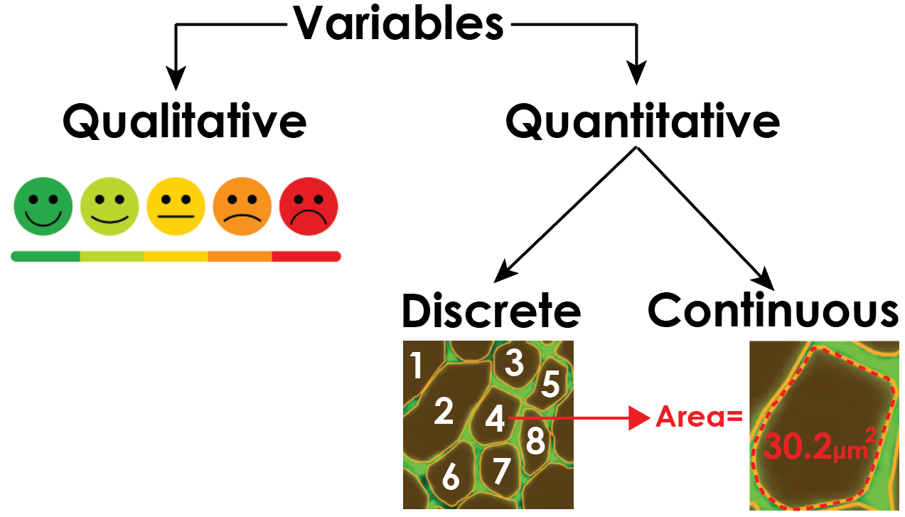
Primarily, variables can be bisected into quantitative and qualitative variables. These broad categories encompass variables that measure and describe data. Quantitative data is represented by a numerical value and represents a measurement of a feature of the data. Qualitative data, conversely, is represented by categories or unstructured responses and offers a high-level description of something.

Qualitative data can serve as a rich source of information. Obtaining such data is useful when the hypothesis is concerned with the complex subjective experience of a subject. For example, qualitative data might be a series of subjective reports on physical response to taking a drug. Although this data is useful, it is incompatible with statistics and thus I will primarily focus on quantitative variables. It is important to note that qualitative data can often be converted into quantitative data. For example, the proportion of patients in the drug group who reported nausea gives a quantitative spin on an otherwise subjectively reported experience.

Quantitative data in biological research aims to represent a biological process or phenomenon as a numerical value. For example, serum cortisol might be measured to infer the stress of a subject and the imaged density of viruses in a cell can inform its infectivity. But what kinds of quantitative variable are there and why are they important?

Discrete vs. Continuous Quantitative Variables

Quantitative variables can be further subdivided into discrete or continuous quantitative variables. Discrete variables are quantitative units of data that have a finite and specified range of potential values. Conversely, continuous variables are quantitative units of data that have a theoretically infinite range of potential values.

In biological research, discrete variables frequently emerge in the form of counts. For example, you might be interested in the number of labeled cells in an image. Since each cell is a singular entity (you can not have .5 of a cell), it constitutes a discrete variable. Continuous variables in biological research are diverse and expansive. In image analysis, these variables typically refer to quantitative metrics of object morphology. For example, of your imaged cells you’ve counted, you might be interested in their cross-sectional area, circularity, or convexity. For image analysis, the pixel intensity of an object can also be an informative continuous quantitative variable. For example, your image might contain fluorophores of antibody-stained tissue where the abundance and intensity of a color reports the quantity of a protein of interest. In this way, pixel intensity and quantity for a biological object can indirectly report molecularly or genetically relevant processes.

Now that we have discussed the types of variables you will encounter when gathering data, how can we begin to understand it?

Descriptive statistics: Quantitatively summarizing your data

When analyzing a set of quantitative data, it is useful to summarize the totality of that data using descriptive statistics. Descriptive statistics aim to, as it’s namesake would suggest, describe three elements of your data: the central tendency, variability, and distribution.

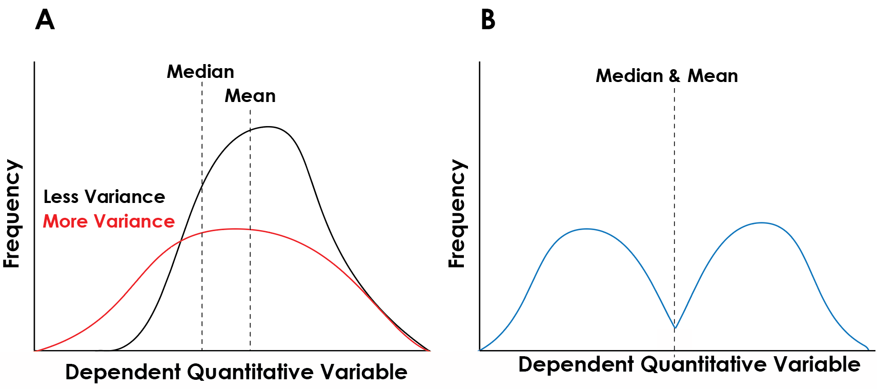
Central tendency: The central tendency of a set of data describes how the totality of the values trend and measures the central and typical values in that data set. The two main measures of central tendency are the mean which represents the average value of the data set and is sensitive to the distribution of data and the median which represents the central most data point and is sensitive to the sample size (Figure 2).

Variability: Whereas the central tendency of a distribution puts forth the average values, the variability of a set of data describes how different the whole distribution is from those average values. In other words. The primary measurement of variability is the standard deviation which represents the average difference between all the points in a data set. A high standard deviation denotes a high variability. This is illustrated in figure 2a. Whereas the mean values for the red and black distributions are similar, the red distribution is more spread out whereas the black distribution is more consolidated around the mean. As such, there are more data points along a greater range of values in the red distribution.

Distribution: As I alluded to above, the distribution refers to how the frequency of certain values of data points are organized across the range of potential values. The distribution is typically illustrated using a histogram (Figure 2) which shows how frequently certain values of data appear in the data set. Distributions come in many shapes (Figure 2). The shape of the distribution is an important characteristic as it tells you how the set of data is structured. Take, for instance, the distribution in figure 2b: The mean and median values are set in the center and the variability is intermediate. The distribution, however, shows two peaks, known as a bimodal distribution. Data distributed in this way typically indicates two subpopulations within your gathered data that might need to be segregates and or might evince a relevant variable you have not considered.

Using Descriptive statistics to compare healthy and diseased muscle tissue

In my previous article on my experience with Biodock’s end to end AI platform, I trained an AI model to perform instance segmentation on muscle fibers in transverse sections of muscle from healthy vs diseased subjects (Figure 3a). Each of these objects can represent a unit of data and within the biodock platform I can extract the cross-sectional area of each collected fiber. I can use statistics of central tendency to show that the population of healthy muscle fibers on average are larger than the diseased muscle fibers (Figure 3b). Next, we can analyze the frequency distribution to determine the relative variability and distribution structure. We find that the diseased fibers have less variability than the healthy fibers as the majority of the observations fall within a smaller range. Interestingly, however, the diseased fibers display a distribution that is skewed to the right whereas the healthy fibers are normally distributed about the mean. This suggests that the diseased fibers have outlier larger fibers within the sample which could correspond to healthy fibers that have yet to succumb to atrophy.

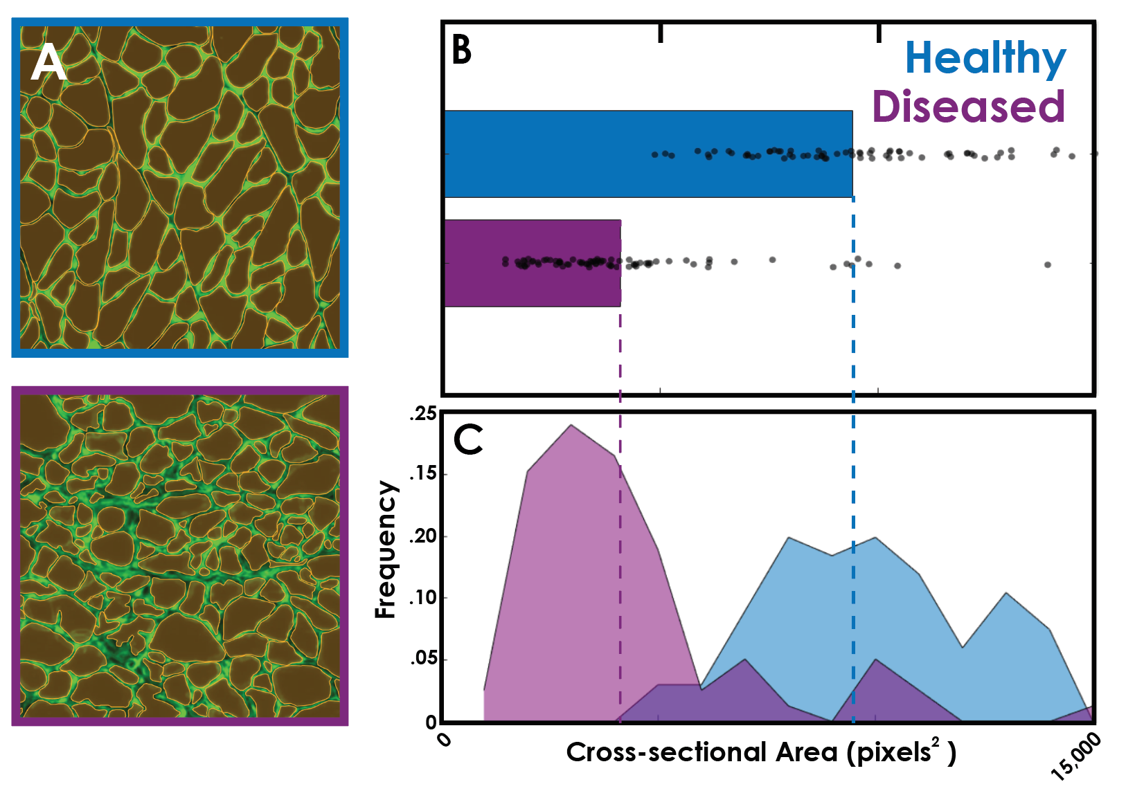
More information on the biological relevance of this image data can be found in my prior article. This offers one example, however, of how descriptive statistics can be used to compare a continuous quantitative variable (area) between biologically distinct conditions and how the nuance of their distributions and variability afford insight into the characteristics of the disease state.

Inferential Statistics: Testing your hypothesis by comparing your sample to the population

The goal of inferential statistics is to understand whether a pattern among your observed data is representative of the population at large. In other words, inferential statistics utilizes the distribution of your data to ‘infer’ the trends beyond your gathered data. Inferential statistics is critical for scientists to validate whether the results they obtain confirm or refute their hypothesis. This branch of statistics bifurcates into two subbranches: parametric and nonparametric. The qualities of the data you are sampling determine the relative inferential statistical methods you should use.

Parametric vs. nonparametric tests

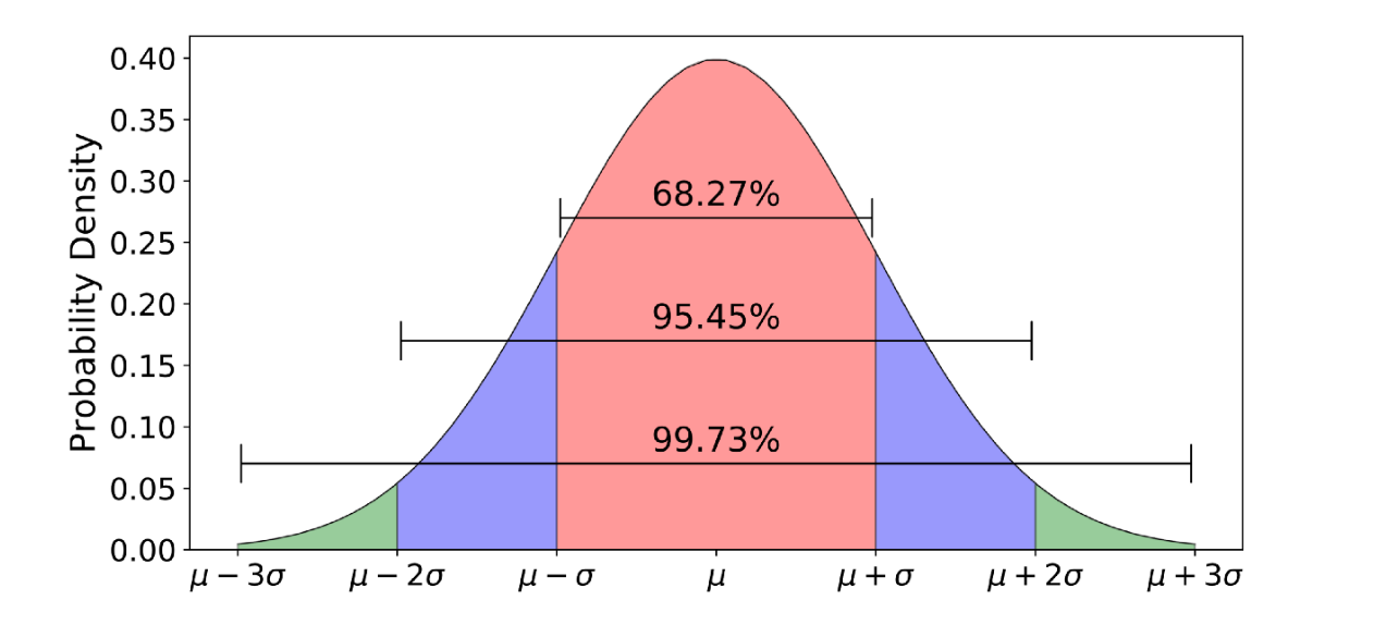
Since inferential statistics aims to generalize to the larger population, tests within this branch are sensitive to the structure of the distribution of the variable you are examining at the population level. This is where understanding your variables and descriptive statistics becomes crucial. Parametric tests make two assumptions: (1) Normality (2) Equal variance. The first assumption relates to how the distribution of data within the population is distributed about the mean. A normal distribution is one where the data is symmetrically clustered about the mean in a bell-shaped curve where each standard deviation from the mean captures progressively less of the data (Figure 4). Examples of normally distributed quantitative variables include height. The second assumption necessitates that the variance of the sample and the population are equal – that is, that how different the values of your observations are from one another should approximate how different they are at the population level. When both assumptions are met, parametric statistical tests may be used. When these assumptions are broken, non-parametric tests must be used. Instances of using non-parametric tests include the population having a skewed distribution.

Parametric and nonparametric tests essentially tell you how likely it is that your observed data is a part or separate from the known population. In this way, you can determine if differences between two groups are due to the contribution of some dependent variable. I will explore this concept in more depth in the forthcoming article. For now, we can generally consider a hypothetical question in cell biology which leverages image analysis and inferential statistics to clarify this point.

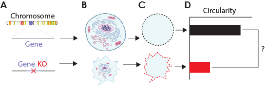
Using inferential statistics to test whether a gene contributes to the polymerization of tubulin

The cytoskeleton serves to maintain the shape and structural integrity of a cell. Microtubules are among the cytoskeletal elements and are comprised of individual monomeric units called tubulin. Polymerization of tubulin to form microtubules is thus a crucial process within cells. Imagine you wanted to use inferential statistics to determine whether a certain gene is involved in the polymerization process. To do this, you culture separate sets of cells where in one dish you have normal cells and, in another dish, you have the same cells, but the gene of interest is knocked out (Figure 5a-b). After staining and imaging these cells you can train a model using biodock to perform instance segmentation on them and obtain their overall structure (Figure 5c). You predict that among the knockout cells, the cytoskeleton will be compromised and so the shape of the cell will become smaller and less circular which can be quantified using continuous quantitative variables such as area and circularity. Assuming that the circularity of these cells is normally distributed and has uniform variance, you can perform a parametric test to determine whether your observed knockout population is misshaped and thus has a defective tubulin polymerization process (Figure 5d). If the assumption of normality and variance are not met, for example if there is another compensatory gene only present in a subset of the population skewing the distribution right, then non-parametric tests can be used to compare the cells.

Conclusions

Statistical methods are powerful and essential tools in science for testing hypotheses. Here, I laid the foundation of descriptive and inferential statistics which serve to outline the structure of data and test the legitimacy of comparisons of that data. These data are comprised of variables whose properties influence how you think about and interact with them and how you choose appropriate statistical tests. These sorts of comparisons and tests, of which some are outlined above, are common when making meaning of biological images. If you are looking to quantify aspects of your image data, Biodock's end to end AI platform streamlines the process of machine learning-based model creation – from labeling to training – and image feature quantification. Reach out to examine all the services Biodock has to offer.