
Recently, Biodock revealed the exciting news that its end-to-end AI platform is coming out of beta testing. Now, versatile, powerful, and user-friendly AI segmentation is readily accessible for scientists to accelerate their image quantification and analysis. As a scientist who has collected and analyzed many images, I am well acquainted with the toil of manual analysis and the impressive potential utility Biodock has to offer. To instantiate this utility, I tried out Biodock myself.
My aim was simple: use real biological images to probe a fundamental research question. In other words, use Biodock to do science. By following the complete workflow of labeling, training, predicting, and analyzing data, I could leverage the ‘end-to-end’ nature of the platform and evaluate its capability. In this article, I formulate a hypothesis-driven research question leveraging image analysis and share my experience using Biodock to answer it.
Table of contents
1. The problem: Quantifying the distribution of muscle fiber area across healthy and dystrophic muscle sections
2. The process: Training an AI model to perform instance segmentation of myofibers
3. The data: What muscle fiber morphology can tell us about the disease
Quantifying the distribution of muscle fiber area across healthy and dystrophic muscle sections
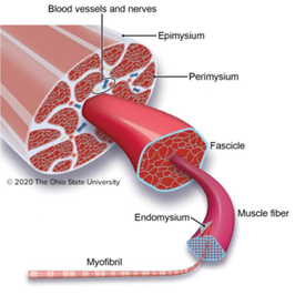
When thinking of an image analysis problem for Biodock to help solve, I turned to the field of muscle biology. Skeletal muscle is composed of a network of organized muscle fibers. Muscle fibers can be further subdivided into a bundle of myofibrils which contain myosin and actin proteins that serve as the contractile units of muscle (Figure 1).
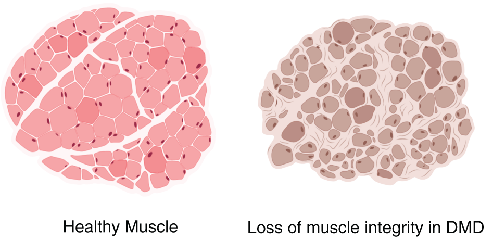
Myofibrils differ in the myosin isoform they express which determines differences in contractile properties and kinetics. Another critical determinant of muscle fiber function is its cross-sectional area (CSA). The larger the fiber the more myofibrils it contains and the greater the force output. Thus, the distribution of cross-sectional area (CSA) is a vital metric in muscle biology since it affords insight into muscle function. Furthermore, CSA is sensitive to physiological changes like exercise and is altered in disease states such as muscular dystrophy (Figure 2).
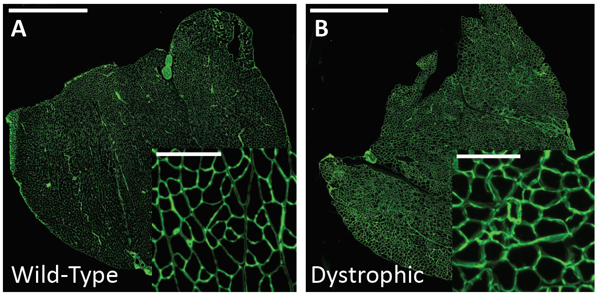
Therefore, routine analysis in muscle biology is to measure the CSA of muscle fibers across treatment and or disease conditions. To do this, the muscle is first dissected and sliced into transverse histological sections. These sections can then be stained for various proteins of interest using immunohistochemistry. Antibodies against laminin, a component of the extracellular matrix, can be used to outline the membrane of muscle fibers (Figure 3a). Then, what is typically done in labs across the country is that each fiber is traced by hand. This is extraordinarily tedious and time-consuming when even small muscles from mice can possess thousands of fibers. This is where Biodock comes in. My goal is to use Biodock to train an AI model that performs instance segmentation on images of laminin-stained muscle fibers to extract the distribution of muscle fiber morphology. I plan to do this across healthy and dystrophic muscle tissues to directly compare how disease state influences the morphology of muscle fibers. Muscular dystrophy is characterized by the atrophy of muscle which leads to small and deformed muscle fibers. Therefore, I hypothesized that the model would demonstrate a difference in the distribution of CSA between healthy and dystrophic muscle tissue. This task is well suited for Biodock’s end-to-end AI platform since I will be able to label, train, predict, and analyze my data all on one platform. In other words, I will be able to test my hypotheses solely using Biodock. The prospect of this is exciting. Not only will I be able to do science all on one platform, but the automated nature of an AI model to outline muscle fibers accelerates and streamlines the science I will do! This contrasts with outlining, measuring, and analyzing all the data myself. Let’s get going.
Training an AI model to perform instance segmentation of myofibers
1: Image Acquisition and Selection
First, I acquired images from the lab of Dr. Hyojung Choo at Emory University. The Choo lab studies the pathophysiology of muscular dystrophy to create targeted therapies. The images are IHC laminin stains of the gastrocnemius muscle from one healthy mouse and another mouse model of limb-girdle muscular dystrophy (Figure 3). From these images, I selected a subset of image inlays to use for labeling.
2: Image labeling
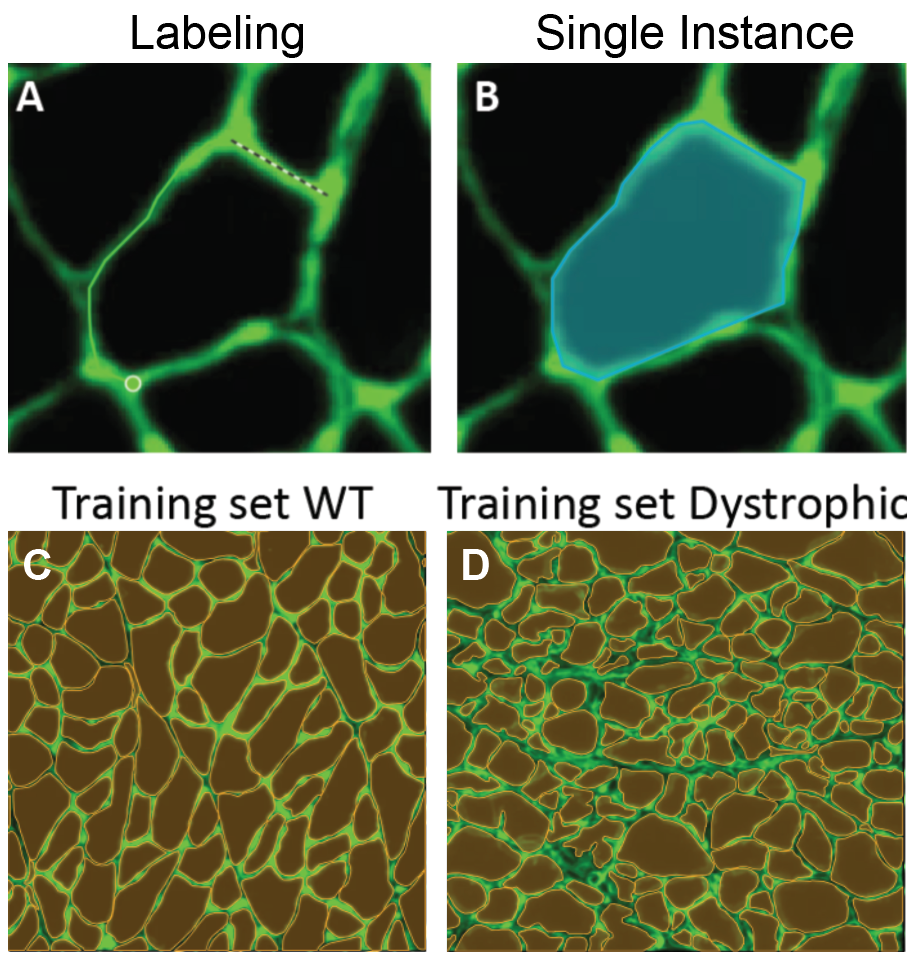
I took five images from each condition (healthy and dystrophic) where four from each condition will be used for labeling and training and the remaining image will be used to test the model. I then imported these into Biodock to start labeling. First, I created a class for muscle fibers and opted for an instance segmentation model. Then, I traced the outlines of all muscle fibers in the section (Figure 4). Importantly, all instances in an image must be labeled for training. If you have high-content images, Biodock will segment cut the image into a grid of smaller images to ease training. Labeling on images from various locations is important since it retains variability, prevents overfitting, and moderates the amount of labeling you do.
3: Training my AI model
Next, I assigned the images to their respective categories of training or test sets. In total, over 1,400 instances of hand-traced fibers were available across the dystrophic and healthy muscle images. To optimize performance of your own model on your data, obtaining as many instances as possible is recommended and depends on the content of the image and the segmentation type. The training for my set took ~5 hours. This should vary depending on your number of classes, instances, and image content.
4: Prediction of muscle fibers on test images
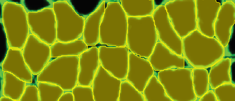
Once my model was ready to run predictions with, I used two test images and ran prediction and analysis (Figure 5a). I was able to obtain the CSA alongside other values for the muscle fibers across healthy and diseased conditions. The quality of the predictions was great. The predictions across both images were nearly perfect (Figure 5a). The model was able to predict equally well across dystrophic and healthy fibers and did not miss muscle fibers. This made for a tiny false-negative rate which is important since some other non-biodock models might systematically miss certain smaller or deformed fibers leading to skewed analysis. Impressively, the false positive rate was also low. This means that what the model was calling a fiber was indeed a fiber. There was no double counting (outlining two fibers) nor erroneous outlines. This is very promising as false positives are typically the more dangerous errors for analysis.
Evaluating the morphological differences between healthy and dystrophic muscle fibers using Biodock AI model
5: Analysis of test images
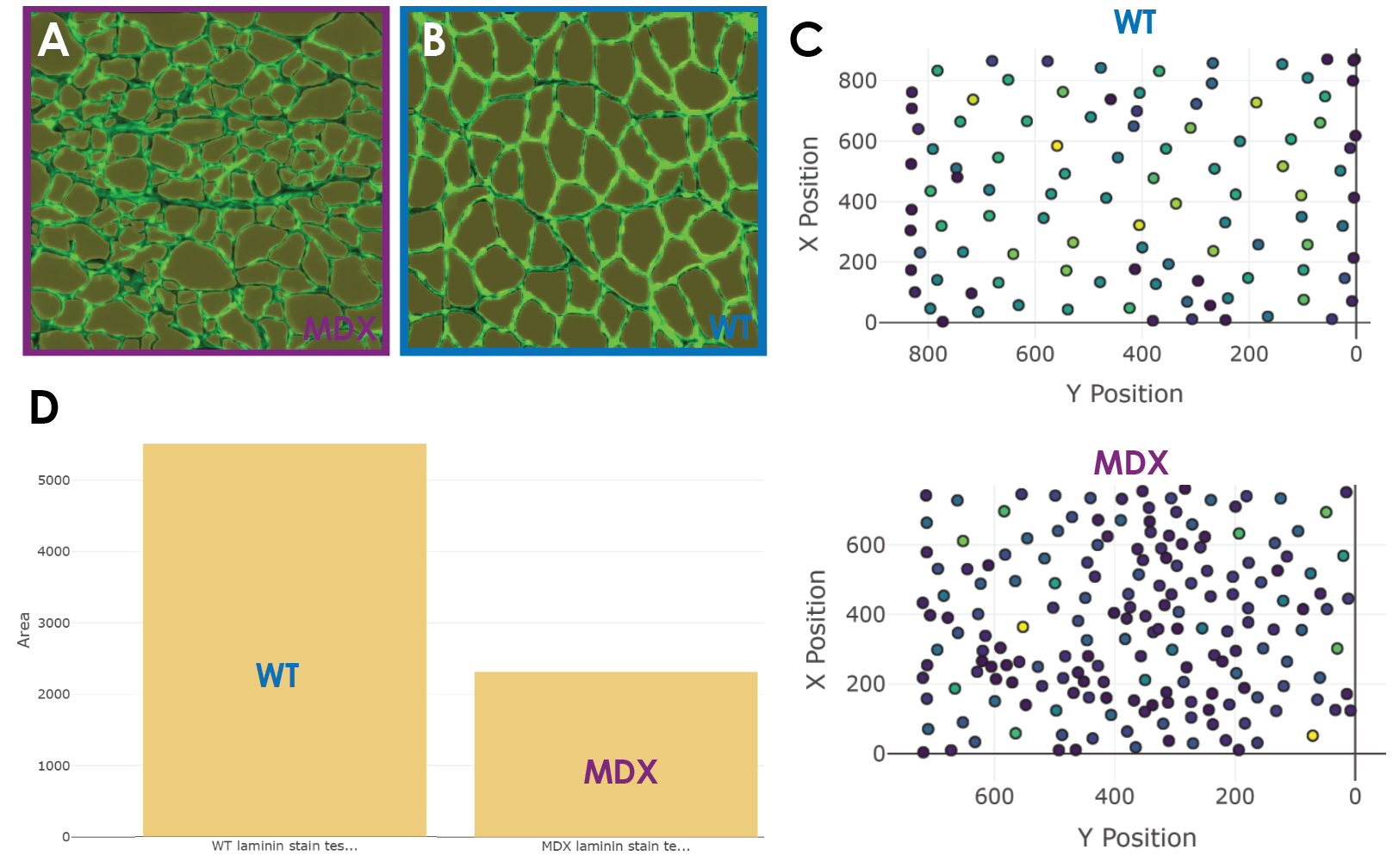
Now that the model was performing adequately, the last step is to compare the distribution of CSA across muscle conditions. Within the Biodock platform, it was easy for me to toggle different quantitative elements of the data to visualize. The scatter plot feature is good for looking at the physical distribution of objects in an image and having them colored by size is a useful feature (Figure 5c). In larger images of muscle, this feature could be used to instantly visualize localized patches of muscle atrophy in dystrophic muscle sections. In fact, these clusters are visible in my data where in the MDX tissue you see more densely packed fibers at a lighter blue color signifying smaller CSA. The histogram feature is useful to examine the distribution of different morphometric units such as area and perimeter. WT fibers are distributed normally and unimodally. Interestingly, the dystrophic fibers seem to be skewed to the right and potentially bimodal. This discrete population of larger fibers are those in the muscle that remain healthy. These healthy fibers are visible in the predictions from the test set. Since muscular dystrophy is a progressive disease, one could use this AI model to perform the same analysis longitudinally. This would likely reveal a shift in the abundance of these fibers and thus a depression in the second distribution as more fibers atrophy. Finally, the bar graph feature was similarly useful in examining gross differences in morphometric units across muscle conditions. Through this, I was directly able to compare the cross-sectional area between healthy and diseased tissue. There is a clear difference in the area of fibers where MDX fibers are characteristically smaller due to atrophy (Figure 5d). The data is also exportable as a .csv and can be opened and analyzed in excel or another software of choice. The file is organized intuitively as a table and is easy to use. I downloaded the file and analyzed the data in MATLAB. I ran a two-sample t-test which showed that the difference in CSA between WT and dystrophic fibers is statistically significant.
Conclusions
Collectively, I was able to train an AI model in Biodock to identify individual muscle fibers that were healthy or atrophied. Through this, I was able to extract and quantify biologically relevant morphological metrics. I found that healthy and diseased fibers constitute separable distributions based on the cross-sectional area, demonstrating the effect of this disease on a metric of muscle function. Although this result was expected, it foreshadows the potential uses for this sort of data, some of which are described above. Importantly, predictions from the model were generated in a matter of seconds whereas manual annotation of the same images would have taken upwards of an hour. Biodock was able to accurately and efficiently accelerate image analysis which led to insight into a hypothesis-driven research question. How’s that for an afternoon of work?