Bioimaging is a well-established and highly effective tool for interrogating biological systems. This broad term refers to the entire process of specimen preparation and staining, raw data acquisition, and data processing/visualization. Although the bioimaging field encompasses the entire range of imaging modalities, including NMR, X-ray, ultrasound, CT, PET, tomography, MRI, and electron microscopy, one of the most common forms of bioimaging in a laboratory setting is fluorescence microscopy. In this article, we’ll focus on the process, practice, and problems associated with setting up, running, and analyzing a fluorescence microscopy experiment.

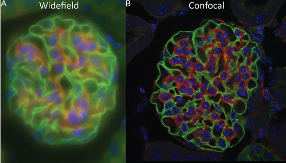
Fluorescence microscopy is one of the most accessible forms of bioimaging for most researchers. Although we won’t go into technical detail on the physical phenomena that make this type of microscopy possible, many great reviews (including this one and this one) exist for those interested in doing a deeper dive. The contrast in fluorescence microscopy is generally excellent relative to other forms of imaging, resulting in a good signal-to-noise ratio and readily interpretable data. With this technique, we can answer questions about biomolecule localization, expression, and kinetics, as well as assess co-localization, structural features, and cellular morphology. The simplest form of fluorescent microscopy is fluorescent widefield microscopy, also known as epifluorescence microscopy, in which the entire field of view is illuminated with excitation light. Epifluorescence microscopy is easy-to-use and fast, and the sample image can be directly observed through the eyepiece. However, this type of scope also tends to generate high background and fluorophore bleed-through when dyes have overlapping emission spectra.

The next step above epifluorescence in terms of complexity and cost is confocal microscopy. In this type of scope, excitation light is emitted by a laser (unlike epifluorescence scopes) at a given focal plane and emission light is focused through a photomultiplier detector pinhole. The use of a pinhole is a major refinement that filters out unfocused light (a cause of blurred images), leading to a better signal-to-noise and image quality over epifluorescence. The ability to take high-resolution images of a specific focal plane as thin as 1 um (termed optical sectioning) also allows us to stitch together a series of focal planes to generate a 3D representation of the sample, pinpoint the location of biomolecules with high confidence, and assess co-localization of different biomolecules. The downsides of this type of microscopy are the greater time costs for training and running the scope—scanning across a sample to acquire images is slow compared to epifluorescence imaging.

Newer forms of fluorescent microscopy improve on resolution and sample penetration, and are appropriate for more specialized imaging applications. Total Internal Reflection Microscopy (TIRF) excites a very thin section (within a few hundred nanometers) of the sample at the coverslip surface corresponding to the air/liquid interface. This type of microscopy can produce very high resolution and high-contrast images of the contact area between the sample and coverslip. On the other hand, 2-Photon Microscopy allows for deeper penetration into thick samples by limiting excitation to a single focal point and using a higher density of lower-intensity light rather than a lower density of high-intensity light. For example, rather than exciting a molecule of GFP with one photon of blue light (as a confocal or epifluorescence scope would), 2-photon scopes use 2 photons of red light. Since long-wavelength red light can travel further into tissues, deeper imaging of focal planes is possible. Finally, lightsheet microscopy uses multiple objectives to create a sheet of light at a given focal plane, illuminating the entire field of view. Originally developed to allow for long-term time-lapse imaging of live biological samples such as developing embryos, this approach is faster than confocal or 2-photon imaging, but is overall less utilized in the biological community due to the expertise needed and DIY nature of most scopes.

Determining which type of microscope and resolution are needed for your particular question is often the starting point for planning an experiment. The two main deciding factors, according to microscopy expert Doug Richardson, director of the Harvard Center for Biological Imaging, are whether you need to image live or fixed samples, and whether you’re looking at thin (<15 μm) or thick (>15 μm) samples. For thin, fixed samples (the most common type of biological imaging), your best options are epifluorescence and confocal. In general, epifluorescence is the way to go unless your imaging needs are one of the following:

- Subcellular localization studies

- Colocalization studies

- Time-lapse imaging

For these applications, confocal microscopy is necessary. Of course, verification of staining and sample prep can be done on an epifluorescence scope first to save time and money before moving to confocal.

If you need to image live cells, the options are a little different. For thin live cell samples (i.e. cell monolayers), epifluorescence is a good option but you may also consider TIRF and 2-Photon microscopy if your needs include optical sectioning and high focal plane resolution or plasma membrane imaging. Thicker live sections (i.e. a live clear zebrafish embryo) present the greatest imaging challenge due to the need for deeper penetration. 2-Photon microscopy was until recently technique of choice here, but lightsheet microscopy is gaining ground. Both techniques allow for optical sectioning and high-contrast images.

For thick fixed samples, the method of choice is confocal microscopy, which can optically section and produce Z-stacks to visualize sample structure over a range of several microns. 2-photon imaging can also be used for this type of sample, and also has the advantage of reducing photobleaching across the sample. Finally, for really large fixed samples which would take unreasonably long to image on confocal or 2-photon scopes, lightsheet microscopes built for large sample imaging are the way to go.

Now that you’ve chosen your imaging modality, you can get started on staining and acquisition optimization! I’ll keep the focus here on fixed samples, as these are the most commonly imaged. In general, the steps involved in sample preparation are as follows:

- Growing biological sample on coverslips

- Fixation

- Permeabilization

- Antibody or dye staining

- Mounting coverslips

All of these steps are possible optimization points, and in general the higher-performance microscope used, the more likely that subpar sample preparation will affect the final image. For an in-depth guide on sample preparation for confocal, epifluorescence, and other types of microscopy, look at this review or this one. Let’s take these steps one-by-one and summarize key pivot points in the optimization process.

Plating samples

In general, growing or differentiating cells directly on a coverslip is the way to go for most applications. The most common coverslip type is the #1.5 coverslip, which has a thickness of 170+/- 10 um. For high-resolution imaging where coverslip thickness variation may pose a problem, high-precision #1.5H coverslips are available, with a margin of error of 5 um. For cell culture, coverslips can be placed directly inside a 24-well plate and lifted out post-sample preparation for mounting, but other options include chamber slides or dishes where #1.5 glass makes up the bottom of the well. The next concern is coverslip coating: some cells cannot stick directly to glass and require a biocompatible coating for sufficient extracellular contacts to form. Options for this include solutions of collagen, poly-L-lysine, and poly-L-ornithine. The best way to determine which biocoating, if any, is necessary for your project is to test out different options and assess the coverslips for cell adherence and resistance to washing away. Adherent cells obviously have an advantage when it comes to imaging, because they naturally put down attachment points and spread out on the coverslip. Non-adherent cells can be spun onto coverslips or adhered to charged coverslip coatings, and other methods such as gravity sedimentation have also been shown to be effective.

Fixation and Permeabilization

The standard for fixation in most labs is paraformaldehyde, either in its pure form or as formalin solution (which also contains methanol). This protocol step should not be one-size-fits-all, however, because different antibodies and stains have incompatibilities with certain fixatives. Methanol and glutaraldehyde are less-used options that nevertheless are optimal for some applications. Some commonly-cited examples include phalloidin labeling, which is incompatible with methanol fixation, and microtubule fixation, which does not work well with formaldehyde. Another pitfall of sub-optimal fixation is reduced antigenicity leading to poor labelling. The length and temperature of fixation also affect the final outcome. A common starting point is 10 minutes at room temperature, and additional modifications can then be made. Permeabilization, typically the next step in a sample preparation protocol, comes with many of the same caveats and pitfalls as fixation. Commonly used perm agents include dilute solutions of the detergents saponin and Triton X-100, incubated for 20 minutes at room temperature. Importantly, saponin permeabilization is reversible, so all subsequent steps must include this reagent.

Staining

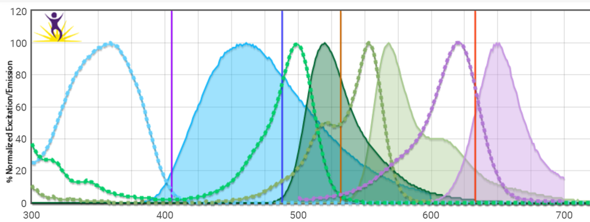
At this step, we sequentially incubate the sample with a dye such as phalloidin (used to label actin filaments) or an antibody to label specific cellular components or biomolecules. Since most of the pertinent information for lengths of time, temperature, and concentration can be found in the user protocol of these different reagents and numerous books and reviews, we won’t go into depth here. A related but critical point here is to know your excitation spectra, emission spectra, and filter sets—some amount of optimization with different fluorophore colors may be necessary to ensure minimal cross-talk or bleed-through of your different colors. Spectral viewers like this one are an excellent way to visualize overlap.

Background autofluorescence may also be a problem for certain fluorophores (particularly green-emitting ones), so running an unstained and set of single-stained controls is good practice in every imaging experiment. Nonspecific staining in the case of antibody labeling is another common pitfall. This can be evaluated by isotype control staining of a parallel sample, and using a blocking agent such as BSA or longer antibody incubation at 4⁰ rather than room temp are possible workarounds.

Now to the microscopy room! Frequent users will be familiar with the “black hole” nature of this room: pitch dark and windowless, it’s just you and the monitor. Many of us have spent countless hours scrolling extremely slowly in the Z axis to find the elusive optimal focus plane, and then countless more hours scrolling through the X/Y plane, playing with laser power, gain, and Z-stack controls to take that perfect image. Each user has their own preferences for image acquisition, but for a beginner it is often helpful to start in conventional brightfield mode on the scope being used to find and focus on the sample being imaged at a relatively low magnification before switching to fluorescence mode. Then, focused on a region of the sample that is non-critical, appropriate gain and laser power settings can be determined. In general, best practice is to use the lowest laser power possible that still gives the desired image in order to avoid photobleaching. The same settings should then be used to image negative controls.

Imaging files are large, but most experienced users prefer to take many more images than necessary and make editing decision during the image analysis step. For heavy microscopy users, this means terabytes of data on an external hard drive or cloud storage. Biodock offers unlimited cloud storage for microscopy images: users can upload image files directly from their browser and download as needed offline access anytime.

Finally, we’ve made it to the last (but not least) step of an imaging experiment: image analysis. The most widely-used processing software is ImageJ, a free open-source program. Fiji, a version of ImageJ packaged along with multiple popular plugins and can read most vendor-specific imaging files, is typically what bioimaging users download. CellProfiler, another free imaging analysis program, is another option which allows you to create your own analysis pipeline and apply it to sets of images. These DIY approaches work well for most users with a small number of samples and the time to devote hours to manually defining settings and running images through analysis steps. However, other commercial alternatives exist—Biodock is one of them! It’s free for academic labs, and our platform will do all the cell identification, quantification, and analysis for you via custom AI-based algorithms. Using our platform ensures maximum reproducibility by eliminating the user bias that comes from manual curation, and saves up to 95% of analysis time. Reach out to us for a consultation and find out how Biodock can transform your imaging journey!